Electric Charges and Fields
Class XII · Physics · Chapter 1 — Coulomb's law, electric fields, dipoles, and Gauss's theorem. The math that runs every phone, lightning strike, and photocopier on earth.
What this chapter is really about 🔉⇢
Rub a balloon on your hair. Now hold it near a thin stream of water from a tap. The water bends. No hands touched it, no wind blew — an invisible thing reached across the gap and pulled. That invisible thing is what this whole chapter is about: the electric field. Once you can draw it, calculate it, and use Gauss's law to short-circuit hard problems, you own the first half of every serious electricity problem in engineering entrance papers.
A charge does not push another charge directly. It first creates a field in the space around it — a real, measurable pattern of force-per-unit-charge — and it is the field that pushes the second charge. Once you replace "action-at-a-distance" with "field first, then force", every problem in this chapter simplifies.
- State and apply Coulomb's law with correct units — including the vector form.
- Sketch electric field lines for a point charge, a dipole, and two like/unlike charges, and read information off them (direction, relative strength).
- Compute the electric field of continuous charge distributions using superposition.
- Apply Gauss's law to derive the field of a sphere, an infinite wire, and an infinite plane in three lines each.
- Handle electric dipoles — moment, field on axial and equatorial lines, torque in a uniform field.
- Solve numerical problems mixing multiple charges without getting the signs wrong.
The 1785 experiment
In 1785, Charles-Augustin de Coulomb hung two tiny charged pith balls from a fine silver wire inside a glass jar, and measured — using the twist of the wire — the force between them as he changed their separation. He found the force fell as $1/r^2$, exactly like Newton's gravity. Two of physics' four forces obey the same inverse-square shape. That similarity is a hint, not a coincidence — but Coulomb didn't know that yet.
Charges are labelled positive (+) or negative (−). Like charges repel, unlike charges attract. In vector Coulomb's law, the unit vector $\hat r_{12}$ points from charge 1 to charge 2 — always. Draw it before you compute. Sign errors are the #1 loss of marks on this topic.
- $e = 1.602 \times 10^{-19}\text{ C}$ — the elementary charge (magnitude on one electron or proton).
- $k = \dfrac{1}{4\pi\varepsilon_0} = 8.99 \times 10^9\,\text{N}\cdot\text{m}^2/\text{C}^2$ — Coulomb's constant.
- $\varepsilon_0 = 8.854 \times 10^{-12}\,\text{C}^2/(\text{N}\cdot\text{m}^2)$ — permittivity of free space.
Core concepts, in the order you'll use them 🔉
1. Electric charge
Two kinds — positive and negative. A neutral atom has equal numbers of protons and electrons. Rubbing a balloon on your hair transfers a few billion electrons; the balloon gets a tiny surplus, your hair a tiny deficit. Charge is quantised — it always comes in integer multiples of $e = 1.602 \times 10^{-19}\text{ C}$ — and it is conserved — the total charge of an isolated system never changes.
2. Coulomb's law (scalar and vector)
The force between two point charges $q_1$ and $q_2$ separated by distance $r$ in vacuum:
Scene 1 of 5 Coulomb force · live 3D 🔉
3. Superposition principle
When many charges act on one, the total force is the vector sum of the pairwise forces. This is why we can handle any complicated arrangement — we just add vectors.
4. Electric field
The electric field at a point is force-per-unit-positive-test-charge placed at that point:
Scene 2 of 5 Electric field at a test point · live 3D 🔉
5. Electric dipole
Two equal and opposite point charges $+q$ and $-q$ separated by a small distance $2a$ form an electric dipole. Its dipole moment is a vector:
Show derivation — dipole field on axial and equatorial line 🔉
Why we care: this is the JEE-level derivation the textbook usually skips. Owning it lets you re-derive the axial : equatorial = 2 : 1 ratio from scratch in an exam — no formula memorisation needed.
Place $+q$ at $x = +a$ and $-q$ at $x = -a$ on the $x$-axis. The dipole moment is $\vec p = q(2a)\hat x$ pointing from $-q$ to $+q$, with $|\vec p| = 2aq$.
Distance from $+q$ to the point $= r - a$. Distance from $-q$ to the point $= r + a$. Both charges' fields lie along $+\hat x$ (from $+q$ pushing outward; from $-q$ pulling inward toward itself, i.e. along $+\hat x$ as seen from the far side).
Actually be careful with signs. Field from $+q$ points away from $+q$, so at a point to the right of $+q$ it points along $+\hat x$. Field from $-q$ points toward $-q$, so at that same right-side point it points along $-\hat x$. So:
$$E_+ = \frac{kq}{(r-a)^2},\quad E_- = \frac{kq}{(r+a)^2}\quad\text{(magnitudes)}$$
Net field (taking $+\hat x$ positive):
$$E_{\text{axial}} = E_+ - E_- = kq\left[\frac{1}{(r-a)^2} - \frac{1}{(r+a)^2}\right] = kq\cdot\frac{(r+a)^2 - (r-a)^2}{(r^2-a^2)^2}$$
Expand the numerator: $(r+a)^2 - (r-a)^2 = 4ar$. So:
$$E_{\text{axial}} = \frac{4kqar}{(r^2-a^2)^2}$$
For a short dipole ($r \gg a$), $(r^2-a^2)^2 \approx r^4$, and $2aq = p$:
Both charges are at distance $\sqrt{r^2+a^2}$ from the point. Magnitudes: $E_+ = E_- = kq/(r^2+a^2)$.
By symmetry, the components along $\hat y$ (radially away from the dipole centre) cancel. What survives is the $\hat x$-component, and both charges' fields contribute in the same direction — opposite to $\vec p$.
The cosine of the angle each field makes with $-\hat x$ is $a/\sqrt{r^2+a^2}$. So:
$$E_{\text{eq}} = 2\cdot\frac{kq}{r^2+a^2}\cdot\frac{a}{\sqrt{r^2+a^2}} = \frac{2kqa}{(r^2+a^2)^{3/2}} = \frac{kp}{(r^2+a^2)^{3/2}}$$
Short-dipole limit ($r \gg a$):
Intuition for the 2 : 1 ratio: on the axis, both charges' fields partially align and reinforce along $\vec p$. On the equator, their fields are tilted and only the small component along the dipole axis survives — the perpendicular parts cancel. Two fields "partly reinforcing" beats "mostly cancelling by geometry".
Physical bonus: both fall as $1/r^3$, not $1/r^2$. That extra power of $r$ is where the "$-q$ nearly cancels $+q$" happens at large distance — you're feeling the difference between two nearly equal 1/r² fields.
6. Electric flux
Flux is how much of a field "pierces" through a surface. If the field is uniform and the area vector $\vec A$ makes angle $\theta$ with $\vec E$:
For a non-uniform field or curved surface, we integrate:
7. Gauss's law
The most powerful shortcut in this chapter:
Dimensional analysis — the mark-saving cheatsheet
| Quantity | Symbol | SI unit | Dimensions |
|---|---|---|---|
| Charge | $q$ | coulomb (C) | [A T] |
| Electric field | $E$ | N/C = V/m | [M L T⁻³ A⁻¹] |
| Coulomb's constant | $k$ | N·m²/C² | [M L³ T⁻⁴ A⁻²] |
| Permittivity | $\varepsilon_0$ | C²/(N·m²) = F/m | [M⁻¹ L⁻³ T⁴ A²] |
| Dipole moment | $p$ | C·m | [L T A] |
| Electric flux | $\Phi_E$ | V·m = N·m²/C | [M L³ T⁻³ A⁻¹] |
If two sides of your final answer don't match dimensions, you have an algebra error somewhere. Check before circling.
3. Contents
This tab is an executive-summary teach of the full chapter — every subsection covered lucidly with a link to the deep-dive. A student reading only this tab comes away with the chapter arc.
See the deep-dive interactive teaching in the linked tab below.
→ Full deep-dive in the overview tabSee the deep-dive interactive teaching in the linked tab below.
→ Full deep-dive in the concepts tabSee the deep-dive interactive teaching in the linked tab below.
→ Full deep-dive in the learnmore tabElectric field lines — see the invisible 🔉
Scene 3 of 5 · flagship Dipole field lines · live 3D · auto-plays 🔉
Michael Faraday didn't have vector calculus. What he had was a bottle of iron filings and a magnet — sprinkle the filings around the magnet and they line up along curves. He argued that space itself had a shape around a charge or magnet, and drew that shape as field lines. His picture is still how every physicist thinks about fields today.
- Lines start on positive charges and end on negative charges (or extend to infinity).
- Tangent to a field line at any point gives the direction of $\vec E$ there.
- Density of lines (lines per unit area perpendicular) is proportional to $|E|$ — packed lines mean strong field.
- Field lines never cross. If they did, $\vec E$ would have two directions at one point — impossible.
- Field lines are continuous curves, no breaks in charge-free regions.
Field-line topology switcher · pick any 2-charge configuration
Coulomb's Law Lab — real numbers, live 🔉
Scene · auto-plays Coulomb force · live 3D · drag q₁, q₂, r 🔉
Drag the sliders. Watch the force change. This is not a cartoon — the computation uses the real Coulomb constant $k = 8.99 \times 10^9$ N·m²/C² and gives you the actual force in newtons. Try to break it: what happens when charges get very close? When one is 0? When one is negative?
Interactive calculator
- Doubling the distance quarters the force (inverse-square).
- Swapping either sign flips the direction from repel to attract.
- Water (κ ≈ 80) reduces the force by 80×. Salt in water screens charges effectively — that's why your cells can function even though they're full of ions.
- At r = 5 cm and q = 1 μC each, the force is already ~3.6 N — comparable to lifting a small apple. Two coulombs at 1 m would be $9 \times 10^9$ N — enough to lift a mountain. That's why you never handle bulk coulombs of charge.
Gauss's law — three-line derivations for hard geometries 🔉
Scene 5 of 5 · flagship Gauss's law · verify Φ = Q/ε₀ for any shape · auto-plays 🔉
Gauss's law says: pick any closed surface (a "Gaussian surface"), add up the flux $\vec E \cdot d\vec A$ through it, and the total equals the enclosed charge divided by $\varepsilon_0$. That's it. The trick is choosing a surface where the field's symmetry lets you pull $E$ outside the integral.
Scene 4 of 5 Electric flux · live 3D · surface chooser 🔉
Show derivation — why Gauss's law follows from Coulomb's law 🔉
Why we care: Gauss's law is stated as though it's an axiom, but it is actually a theorem — a consequence of Coulomb's law plus the geometry of solid angles. If you understand the derivation, you understand why $1/r^2$ is the only power that would make Gauss work — no other exponent survives the area-vs-radius cancellation.
Put a point charge $q$ at the centre of a sphere of radius $R$. Coulomb tells us $\vec E$ points radially outward with magnitude $E = kq/R^2 = q/(4\pi\varepsilon_0 R^2)$, the same everywhere on the sphere. The area vector $d\vec A$ is also radially outward, so $\vec E \cdot d\vec A = E\,dA$. Total flux:
$$\Phi = \oint \vec E \cdot d\vec A = E \cdot (4\pi R^2) = \frac{q}{4\pi\varepsilon_0 R^2}\cdot 4\pi R^2 = \frac{q}{\varepsilon_0}$$
Notice: $R$ vanished. The $4\pi R^2$ growth of surface area exactly cancels the $1/R^2$ decay of the field. That cancellation is only possible because Coulomb's law is inverse-square. If the force were $1/r^3$, we'd have leftover $R$ in the answer and Gauss wouldn't be radius-independent.
Deform the sphere into any closed surface $S$ still enclosing $q$. For any small patch $d\vec A$ at distance $r$ from the charge, the projection perpendicular to $\vec E$ is $d\vec A\cdot\hat r = dA\cos\theta$. Flux through the patch:
$$d\Phi = \frac{kq}{r^2}\,dA\cos\theta = kq\cdot\frac{dA\cos\theta}{r^2} = kq\cdot d\Omega$$
where $d\Omega = dA\cos\theta/r^2$ is the solid angle the patch subtends at the charge. Integrating over the whole closed surface, the solid angle is $4\pi$ (that's just the definition — a closed surface enclosing a point subtends the full sphere of directions). So:
$$\Phi = kq \cdot 4\pi = \frac{q}{\varepsilon_0} \quad \text{(surface-shape independent)}$$
For a charge outside the surface, every field line that enters must also exit (the surface is closed). Inward flux and outward flux cancel exactly. Net contribution to $\Phi$: zero. So only enclosed charges matter.
For many charges $q_1, q_2, \ldots$ (some inside, some outside), the total field is the sum of individual fields (superposition). Flux is linear in field. So:
$$\Phi_{\text{total}} = \sum_{i \in \text{inside}} \frac{q_i}{\varepsilon_0} + \sum_{i \in \text{outside}} 0 = \frac{Q_{\text{enclosed}}}{\varepsilon_0}$$
Gauss's law is not a new physics postulate. It is Coulomb's law repackaged so you can exploit symmetry. The strength of the packaging is that once you have the right Gaussian surface, evaluating $\oint \vec E \cdot d\vec A$ becomes trivial — you avoid the ugly integrals you'd need with pure Coulomb superposition.
Case 1 — Field of a point charge (spherical Gauss surface)
By symmetry, $\vec E$ is radial and has the same magnitude everywhere on a sphere of radius $r$ around the charge. So:
Case 2 — Infinite line charge (cylindrical Gauss surface)
Charge per unit length $\lambda$. Cylinder of radius $r$, length $L$. By symmetry, $\vec E$ is radial (perpendicular to the wire) and constant on the curved surface; zero flux through the flat ends.
Show derivation — infinite-line E-field, step by step 🔉
Why we care: this is the workhorse of every cable, capacitor-plate edge, and transmission-line calculation. If you cannot re-derive $E = \lambda/(2\pi\varepsilon_0 r)$ from Gauss without the textbook, you'll blank on the JEE 3-mark problem where they twist the geometry slightly.
Line of charge, infinite in extent, uniform linear density $\lambda$ (C/m). What does the field look like?
- Translational symmetry along the wire: the field cannot depend on which point along the wire's axis you pick. It has no $z$-dependence.
- Rotational symmetry around the wire: the field cannot depend on the angle $\phi$. It has no $\phi$-dependence.
- Reflection symmetry through the wire's midplane: no component along the wire (the $z$-component from charge above cancels the $z$-component from charge below).
Conclusion: $\vec E$ points radially outward from the wire, and its magnitude depends only on $r$ (the perpendicular distance). Write $\vec E = E(r)\,\hat r$.
Take a cylinder of radius $r$ and length $L$ coaxial with the wire. Three pieces of surface: the curved side, and two flat ends (top and bottom).
- Curved side: $\vec E$ is radial, $d\vec A$ is radial (points outward from the cylinder's axis). So $\vec E \cdot d\vec A = E(r)\,dA$, and $E(r)$ is constant on this whole surface. Total flux: $E(r) \cdot (2\pi r L)$.
- Flat top and bottom: $d\vec A$ points along $\pm\hat z$; $\vec E$ has no $\hat z$ component. So $\vec E \cdot d\vec A = 0$. No contribution.
Length $L$ of wire is inside the cylinder, so $Q_{\text{enc}} = \lambda L$.
$$E(r) \cdot 2\pi r L = \frac{\lambda L}{\varepsilon_0}$$
The $L$ cancels — as it must, because our answer cannot depend on the arbitrary length of the Gaussian cylinder:
The $1/r$ (not $1/r^2$) is not a bug. Every length element $d\ell$ of the wire contributes $dE \propto 1/r^2$, but you integrate over an infinite line — one power of $r$ is "eaten" by the fact that the source extends to infinity along one dimension. Same reason infinite plane gives $r^0$ (independent of distance) — two dimensions of source eat both powers of $r$.
Students sometimes try to use a sphere as the Gauss surface here. Won't work: on a sphere, $\vec E$ is not constant in magnitude ($r$ varies from point to point on a sphere centred on the wire) and not always perpendicular to the surface. You lose the "$E$ comes out of the integral" trick — and the whole point of Gauss is that trick. The Gaussian surface must match the symmetry of the source.
Case 3 — Infinite plane sheet (pillbox surface)
Surface charge density $\sigma$. Pillbox with area $A$ on each face. By symmetry, $\vec E$ is perpendicular to the plane, equal on both sides.
Students memorise "$E = \sigma/\varepsilon_0$ for a plane" and lose marks because that formula is only for a conducting sheet (charge on one face). A non-conducting sheet has $\sigma/2\varepsilon_0$. Read the problem — is the sheet a conductor or an insulator?
Worked examples — see the full solution, then try it yourself 🔉
Every problem here is a mini template you can copy for entrance-exam numericals. Read the "Given / Find / Solution" pattern until you own it.
Example 1 — Force between two point charges
Example 2 — Superposition of three charges
Example 3 — Electric field of a dipole on the axial line
Example 4 — Gauss's law on a uniformly charged sphere
Example 5 — Torque on a dipole
JEE Advanced — 3 problems that combine ideas
Example 6 — Charged arc on the axis (JEE Adv template)
Example 7 — Two shells, Gauss + superposition (JEE Adv, 3-marker)
Example 8 — Cavity in a solid uniformly-charged sphere (JEE Adv, elegant)
Conceptual traps — see the wrong answer, then the right one
Trap 1 — "$E = \sigma/\varepsilon_0$" versus "$E = \sigma/(2\varepsilon_0)$"
Trap 2 — "Charge outside a Gaussian surface contributes to the field on the surface, so the flux must depend on it"
The people behind the equations 🔉
Every formula in this chapter is somebody's hard-won insight. Their names got attached because they answered a specific question that had bothered physicists for decades. Reading them in order shows electrostatics being built brick by brick over 80 years.
1785 → 1837 → 1873 — three thinkers, three ideas, one theory
Portraits sourced from Wikimedia Commons, all in the public domain. Credits stored in assets/portraits/*.credit.txt.

In 1785 Coulomb built a torsion balance — two pith balls hanging from a thin silver wire in a glass jar. When he charged them, the wire twisted; the twist angle measured the force. Varying the distance, he found force $\propto 1/r^2$ across two decades of separation. He then locked in the sign rules (like charges repel, unlike attract) and produced the equation that carries his name. His paper, "Premier mémoire sur l'électricité et le magnétisme", is the birth certificate of quantitative electrostatics.
Portrait: Louis Hierle, 1894 · Wikimedia Commons · Public domain

Faraday had almost no formal mathematics — he was a bookbinder's apprentice who taught himself science. But he had geometric imagination. In the 1830s, watching iron filings arrange themselves around magnets, he insisted that space itself carried a state — what he called lines of force. His notebooks show the field-line picture before anyone could write $\vec E(\vec r)$ down. Later mathematicians (Maxwell first among them) gave the picture equations. Every arrow you draw in this chapter is Faraday's ghost.
Portrait: Thomas Phillips, 1841-1842 · Wikimedia Commons · Public domain

Gauss, already famous for the number-theoretic and geodetic Gauss, turned to electromagnetism in the 1830s. He wrote down what we now call the flux theorem: for any closed surface, the total electric flux equals the enclosed charge over $\varepsilon_0$. It followed from Coulomb by the solid-angle argument — no new physics — but it gave you a way to compute $\vec E$ in symmetric geometries in three lines instead of thirty. Maxwell adopted it as one of his four equations. Every high-symmetry electrostatics problem you will ever solve routes through Gauss's shortcut.
Portrait: Christian Albrecht Jensen, 1840 · Wikimedia Commons · Public domain

In 1861-65 Maxwell wrote down four equations that packaged everything Coulomb had measured, Faraday had drawn, and Gauss had computed into one coupled system. Gauss's law became "Maxwell equation I" — the first line of the unified theory. Later he realised his own equations predicted electromagnetic waves travelling at exactly the measured speed of light. Electricity, magnetism, and light — one phenomenon. This chapter is where that story starts.
Portrait: George J. Stodart, c.1870s · Wikimedia Commons · Public domain
- Coulomb (1785) tells you the force law between two charges — but leaves the "how do they know?" question unanswered.
- Faraday (1830s) answers it with a picture: the field is real, it fills space, and the second charge responds only to the field at its location.
- Gauss (1830s) notices that Faraday's picture plus Coulomb's law gives a bookkeeping identity — the flux theorem — that turns hard geometry into easy geometry.
- Maxwell (1860s) writes all of it as one system of equations and predicts electromagnetic waves.
You are not learning four disconnected formulas. You are re-tracing 80 years of insight, in the order it happened.
Learn More — curated sources beyond this chapter 🔉
If a section here didn't land — or you want more depth — here are hand-picked sources. Every link points to a specific moment, not just a homepage. English and Hindi both represented.
🔊 Audio-first explainers (put in earbuds during a walk)
📺 YouTube deep-dives — timestamped to the exact moment

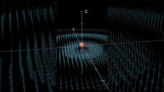

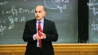
Vfp4kR-tXlE, verified 404 on 2026-07-19) with Yale's canonical Gauss lecture — same rigor, plus the shell-theorem/solid-angle argument in the first half. Verified live via oEmbed 2026-07-19.
📚 Written references — the reading ladder
Every URL above was verified to exist as of 2026-07-15 IST. Timestamps are agent-authored best-guesses; run the video-indexer against each to lock exact ranges.
Dive Deeper — beyond the syllabus 🔉
Everything below is optional for the boards, but any one of these sections will make you noticeably stronger on JEE Advanced — and is where the "future physicist" separates from the "syllabus completer".
A1. Feynman Vol II compressed into an animation — solid-angle proof of Gauss's law
Feynman Volume II Chapter 4 §4-5 proves Gauss's law from Coulomb + solid angles in about 3 pages. Below is the same argument in one picture: a floating charge inside two very different closed surfaces, both giving the same flux $q/\varepsilon_0$.
A2. Null-point locator — where $\vec E = 0$ between two like charges
A JEE favourite: two like charges $Q$ and $q$ ($Q > q$) on the $x$-axis, separated by $d$. Between them, at distance $x = d/(1+\sqrt{q/Q})$ from $Q$, the fields cancel exactly — closer to the smaller charge, because a smaller charge needs less distance to match a bigger one's field.
A3. Dipole field vectors — why axial : equatorial = 2 : 1
The 2 : 1 ratio is not a coincidence — it falls out of vector addition. On the axis both fields partially reinforce; on the equator both fields tilt and only the component along $\vec p$ survives.
A4. Gaussian pillbox — why the flat sheet gives $E = \sigma/(2\varepsilon_0)$
The pillbox has area $A$ on each face. Flat top and bottom see the same magnitude of $\vec E$ pointing outward on each side — two face contributions, one enclosed sheet.
A5. $E(r)$ inside vs outside a uniformly-charged solid sphere
Combines both worked-example answers into one plot. Inside: $E \propto r$. Outside: $E \propto 1/r^2$. Peak at the surface $r = R$; continuous but with a kink in slope.
B. Web-sourced depth — proofs, controversies, subtleties
- Gauss's law — Wikipedia: integral and differential forms, proofs from Coulomb and from Maxwell.
- Coulomb's law — Wikipedia: actual experimental history — Coulomb's original data was not as clean as textbooks suggest.
- Physics.SE — why $E = \sigma/(2\varepsilon_0)$ for a non-conducting sheet: three derivations, one result.
- Physics.SE — Gauss's law in differential-form language: how modern geometric mathematics packages Maxwell into two equations.
- authoritative Physics Part I Ch 1 (free PDF): syllabus source-of-truth for syllabus-approved.
- Feynman Vol II Ch 4: derives Coulomb from Gauss — inverts textbook order.
- OpenStax University Physics Vol 2: free CC-BY textbook, more problems.
- Torsion balance — Wikipedia: Coulomb's apparatus, later used by Cavendish (gravitation) and Eötvös (equivalence principle).
- Millikan oil drop — Wikipedia: how the charge $e$ was actually measured, plus the rejected-data controversy.
- Michael Faraday — Wikipedia: the self-taught bookbinder who invented the field concept before it had equations.
C. Timestamped video moments — the exact scene worth watching
D. Reading ladder — six months from now, in this order
- Week 1: authoritative Ch 1 → solve every exercise.
- Week 2: H. C. Verma Concepts of Physics Vol 2 Ch 29 → all JEE-standard problems.
- Week 3: Halliday–Resnick Ch 21-23 → problem variety + rigorous notation.
- Week 4: Feynman Vol II Ch 4-5 → derives Coulomb from Gauss, reverses textbook order.
- Month 3: Griffiths, Introduction to Electrodynamics 4e Ch 2 → divergence + curl of $\vec E$.
- Month 6: Jackson, Classical Electrodynamics Ch 1 (grad-level). Only if you're still curious.
E. Real-world case studies — where these equations pay rent
- Xerox / laser printer: photoconductive drum holds a $\sigma$-distribution matching your document; toner particles feel Coulomb forces from that surface field.
- Lightning rod: sharp conductor concentrates surface density (curvature $\uparrow$ → $\sigma \uparrow$), boosting $E$ past the air-breakdown threshold ($3\times 10^6$ V/m).
- MRI gradient coils: designed via Gauss's law + boundary conditions on cylindrical geometries — the magnetic dual of $E = \lambda/(2\pi\varepsilon_0 r)$.
- Neuronal ion channels: $\sim 70$ mV across $\sim 5$ nm membranes gives $E \approx 10^7$ V/m — fires every action potential in your brain.
- Van de Graaff / particle accelerator: stores charge on a hollow spherical dome; by Gauss, $E = 0$ inside — hence a person can stand on a 5-MV dome and not die.
F. Open questions — what physicists still argue about
- Is charge exactly quantised in units of $e$? Free quarks are never observed. Limits: no sub-$e$ charge to 1 part in $10^{21}$.
- Is Coulomb's law exactly $1/r^2$? Any deviation would imply a photon mass. Current limit: $m_\gamma < 10^{-18}$ eV; exponent deviation $|\epsilon| < 10^{-16}$.
- Do magnetic monopoles exist? Maxwell says no ($\oint \vec B \cdot d\vec A = 0$). GUTs predict them at very high energies. None observed.
- Does the electron have structure below $10^{-19}$ m? High-energy scattering says no. If it does, Coulomb's law breaks at those distances.
Do not read Dive Deeper in order like a lecture. Pick one section that catches your eye today, follow it end-to-end (video → article → problem), then close the tab. Come back tomorrow.
Assessment — 5 questions, 15 minutes 🔉
Before you take the quiz — 5 lines you should remember 🔉
- 🔉 Coulomb's law is $F = k\,q_1q_2/r^2$ — inverse square, signs matter, superpose vectorially.
- 🔉 Electric field $\vec E = \vec F / q_0$ is force per unit positive test charge — a vector at every point in space, with $\hat r$ pointing away from a positive source.
- 🔉 Field lines start on +, end on −, never cross, and their density gives $|E|$. Any 2-charge sketch reduces to combinations of these rules.
- 🔉 For a short dipole $\vec p$: axial field $E = 2kp/r^3$ along $\vec p$; equatorial $E = kp/r^3$ opposite to $\vec p$. Ratio $= 2 : 1$. Torque in a uniform field $\vec\tau = \vec p \times \vec E$.
- 🔉 Gauss's law $\oint \vec E \cdot d\vec A = Q_{\text{enc}}/\varepsilon_0$ turns hard problems into three-line derivations when the symmetry is right — sphere for point/shell, cylinder for line, pillbox for plane.
Opt-in only. Shows first name, city, and score. Change your mind anytime — data lives on this device.
🏆 Hall of Fame
- 🥇 Priya S. · Delhi · DPS RK Puram — 5/5 (bonus 5) · seed
- 🥈 Aarav K. · Bengaluru · Bishop Cotton — 5/5 (bonus 4) · seed
- 🥉 Meera R. · Kochi · Vidyodaya School — 5/5 (bonus 3) · seed
🕹️ Now YOU teach it
Featured submissions
A 60-second stop-motion where a viewer walks away from a big charged wall. Every step, more charge comes into view from the sides — exactly compensating the $1/r^2$ falloff of any single element. Punchline: "flat = infinite = uniform".
A four-bar rap that walks Gauss's law from Coulomb: "One over r-square is the field / area is r-square, they cancel and yield / four-pi q over epsilon-nought / any surface, any shape, that's what Gauss taught". Ships as an 8-panel comic strip.
A poster split diagonally: left half shows a point charge with an arrow "E halves when r doubles"; right half shows an infinite sheet with an unchanging arrow at every distance. Caption: "one dimension of source per power of r".
JEE / NEET — 8 tier-tagged problems
Tier-tagged questions modelled on real JEE Main / Advanced / NEET-UG patterns. Each has a worked-out solution — read it only after attempting.
Q1. Two identical conducting spheres carry charges +7q and −q. They are brought into contact and then separated to their original distance r. The ratio of the new force to the original force between them is:
💡 Solution
Q2. The electric field on the axis of a short dipole at distance r is E₁. The field on its equatorial line at the same distance is E₂. The ratio E₁ : E₂ equals:
💡 Solution
Q3. A point charge Q sits at the exact centre of a cube of side a. What is the electric flux through one face of the cube?
💡 Solution
Q4. Two infinite parallel non-conducting planes carry uniform surface charge densities +σ and +2σ. The electric field magnitude in the region between the two planes is:
💡 Solution
Q5. Three point charges +q, +q, and Q lie in a straight line, the two +q charges at the ends of a segment of length L and Q at the midpoint. For Q to keep the entire system in equilibrium, Q must equal:
💡 Solution
Q6. An electric field E = 200 î N/C exists in space. The flux through a square of side 20 cm whose plane is oriented so that its normal makes an angle of 60° with the x-axis is:
💡 Solution
Q7. An electric dipole of moment p is placed in a uniform electric field E. Which of the following is true about the torque and potential energy of the dipole?
💡 Solution
Q8. A thin ring of radius R carries a uniform charge Q. The electric field on the axis of the ring is maximum at an axial distance: